K-Means Clustering with Python — Beginner Tutorial

Sorry, no opening. I assume you already know what’s clustering and what the purpose of this thing, so let’s jump straight to the tutorial.

Or if you still confused about the definition and the purpose of clustering in data analysis, you can check out this link: https://developers.google.com/machine-learning/clustering/overview

Import the library.

import pandas as pd  
import numpy as np  
import matplotlib.pyplot as plt  
from sklearn.cluster import KMeans  
from sklearn import datasets

Load the dataset.

iris = pd.read_csv('iris.csv')

Yeah, we’re going to use the iris dataset. It’s a pretty good dataset for beginner purposes to learn machine learning.

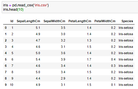
If you take a look at the data on column ‘Species’, there is some kind of extra string (Iris-) before the species name. Let’s delete the extra string, we can do it like this:

iris['Species'] = iris.Species.str.replace('Iris-' , '') 

Now we get more clean species name string.

Substract the values.

To do the clustering we only need four features (sepal length, sepal width, petal length, and petal width) from the table. So we can substract these columns into new variable called ‘x’.

x = iris.iloc[:, [1,2,3,4]]

After substract the columns, now we want to substract the values into an array table using numpy array function.

x  = np.array(x)

Find the optimal number of clusters.

So, before we implement the k-means and assign the centers of our data, we can also make a quick analyze to find the optimal number (centers) of clusters using Elbow Method.

# Collecting the distortions into list  
distortions = []  
K = range(1,10)  
for k in K:  
 kmeanModel = KMeans(n_clusters=k)  
 kmeanModel.fit(x)  
 distortions.append(kmeanModel.inertia_)# Plotting the distortions  
plt.figure(figsize=(16,8))  
plt.plot(K, distortions, ‘bx-’)  
plt.xlabel(‘k’)  
plt.ylabel(‘Distortion’)  
plt.title(‘The Elbow Method showing the optimal clusters’)  
plt.show()

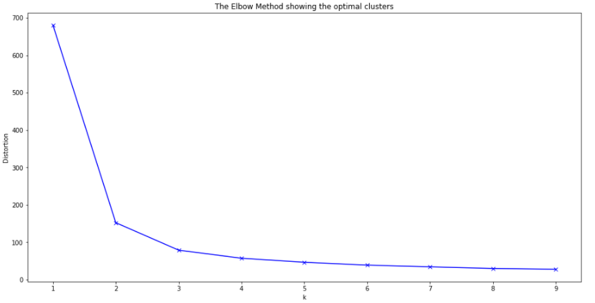
From the line-chart above, we can observe that the “elbow” is the number 3 which is the optimal clusters (center) in this case.

Implement the K-Means.

# Define the model  
kmeans_model = KMeans(n_clusters=3, n_jobs=3, random_state=32932)  
# Fit into our dataset fit  
kmeans_predict = kmeans_model.fit_predict(x)

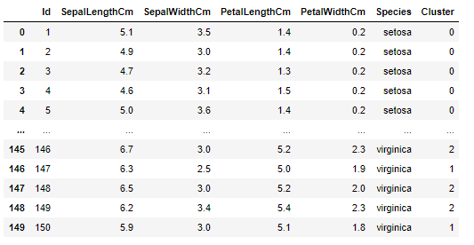
From this step, we have already made our clusters as you can see below:

3 clusters within 0, 1, and 2 numbers. We can also merge the result of the clusters with our original data table like this:

iris['Cluster'] = kmeans_predict

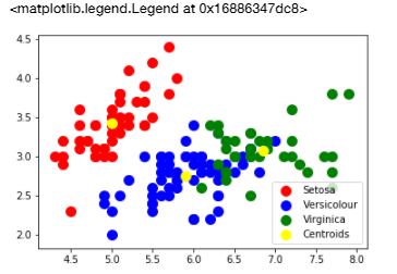
The final step and most necessary step is to visualize our clusters so we can actually see the model of the clusters.

Visualize the clusters.

# Visualising the clusters  
plt.scatter(x[kmeans_predict == 0, 0], x[kmeans_predict == 0, 1], s = 100, c = ‘red’, label = ‘Setosa’)  
plt.scatter(x[kmeans_predict == 1, 0], x[kmeans_predict == 1, 1], s = 100, c = ‘blue’, label = ‘Versicolour’)  
plt.scatter(x[kmeans_predict == 2, 0], x[kmeans_predict == 2, 1], s = 100, c = ‘green’, label = ‘Virginica’)# Plotting the centroids of the clusters  
plt.scatter(kmeans_model.cluster_centers_[:, 0], kmeans_model.cluster_centers_[:,1], s = 100, c = ‘yellow’, label = ‘Centroids’)plt.legend()

Summary

• Clustering in the most common form of unsupervised learning, which the data is unlabeled involves segregating data based on the similarity between data instances.
• K-means is a popular technique for clustering. It involves an iterative process to find cluster centers called centroids and assigning data points to one of the centroids.
• The steps of K-means clustering include:
  1. Identify number of cluster K
  2. Identify centroid for each cluster
  3. Determine distance of objects to centroid
  4. Grouping objects based on minimum distance

The notebook is available here: K-Mean’s Notebook