I’m a fan of Fleet Foxes. I’ve known them since not for so long; I remember stumbled upon their hit ‘Blue Ridge Mountains’ on Spotify and since that time the track, the album and the band become my all-time favorites.
The one thing that I like about Fleet Foxes is their lyrics is always have a deep meaning and sometimes can drive me into an eternal space of refreshment. Their lyrics is full of energizing vibe and tone, but on the other hand, their lyrics also can become so full of sadness and worries.
In this article, I want to explore more about five of Fleet Foxes’s song. I want to know how they built up the tone and the vibe from each piece of word which they arranged to become a perfect melody. I will use five songs: Blue Ridge Mountains, Ragged Wood, Mykonos, White Winter Hymnal and Helplessness Blues.
The first thing I need to do is preparing the tools, which is all the packages that can facilitate me to do this analysis.
Load the package.
library(genius)
library(tm)
library(tidyverse)
library(tidytext)
library(magrittr)
library(wordcloud)
library(syuzhet)
library(igraph)
library(ggraph)
library(readr)
library(circlize)
library(reshape2)
If you see, I’m using a genius package to import the lyrics of the song from Genius website. It’s a pretty good package so I don’t have to copy and paste the lyrics into a file anymore.
Import the data.
song1 <- genius_lyrics(artist = "Fleet Foxes", song = "Blue Ridge Mountains") %>% mutate(artist= "Fleet Foxes")
song2 <- genius_lyrics(artist = "Fleet Foxes", song = "Mykonos") %>% mutate(artist= "Fleet Foxes")
song3 <- genius_lyrics(artist = "Fleet Foxes", song = "White Winter Hymnal") %>% mutate(artist= "Fleet Foxes")
song4 <- genius_lyrics(artist = "Fleet Foxes", song = "Helplessness Blues") %>% mutate(artist= "Fleet Foxes")
song5 <- genius_lyrics(artist = "Fleet Foxes", song = "Ragged Wood") %>% mutate(artist= "Fleet Foxes")
all_song <- song1 %>% bind_rows(song2) %>% bind_rows(song3) %>% bind_rows(song4) %>% bind_rows(song5)
Once I have completely gathered all of five songs, then the next thing I want to do is counting the words from the each songs.
Count the words.
all_song$length <- str_count(all_song$lyric,"\S+")all_song_count <- all_song %>% group_by(track_title, artist) %>%
summarise(length= sum(length))
After that, I visualize the data using barchat.
all_song_count %>%
arrange(desc(length)) %>%
slice(1:10) %>%
ggplot(., aes(x = reorder(track_title, -length), length, fill = artist)) +
geom_bar(stat= 'identity') + # , fill= "#EF504D"
ylab("Word count") + xlab("Track title") +
ggtitle("Amount of words from each songs") +
theme_minimal()
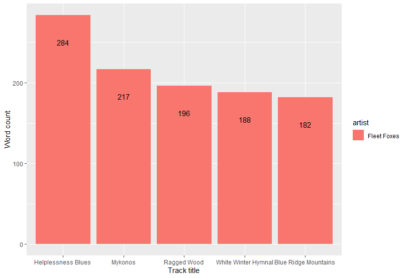
As you see, Helplessness Blues is actually has a lot of words more than four other songs. The next thing I want to know is the variety (diversity) of the word from each songs.
Throw the repetitive word to make it unique for each songs.
tidy_lyrics <- all_song %>%
unnest_tokens(word,lyric)word_diversity <- tidy_lyrics %>%
group_by(artist,track_title) %>%
summarise(word_diversity = n_distinct(word)) %>%
arrange(desc(word_diversity))
Then, visualize it.
word_diversity %>%
ggplot(aes(reorder(track_title, -word_diversity), word_diversity)) + geom_bar(stat = "identity", fill = my_colors) +
ggtitle("Score of diversity of the word from each songs") +
xlab("Track Title") +
ylab("") + geom_text(aes(label = word_diversity, vjust = 5)) +
scale_color_manual(values = my_colors) + theme_classic()
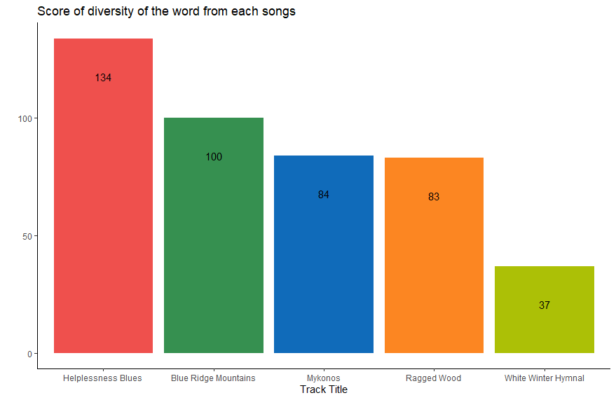
After I throw the repetitive words and make it all unique (only one), as you see, Blue Ridge Mountains become the runner up while White Winter Hymnal fall to the last one.
Next thing, I want to know the most used words from the five songs. To do this, I have to transform the data (lyrics) and make it as clean as possible, so I could sort which word has the largest frequency.
Make it tidy.
docs <- tidy_lyrics$word
docs <- Corpus(VectorSource(tidy_lyrics$word))
toSpace <- content_transformer(function (x , pattern ) gsub(pattern, " ", x))
docs <- tm_map(docs, toSpace, "/")
docs <- tm_map(docs, toSpace, "@")
docs <- tm_map(docs, toSpace, "'")
docs <- tm_map(docs, toSpace, "'")
docs <- tm_map(docs, toSpace, "\|")
docs <- tm_map(docs, content_transformer(tolower))
myStopwords <- stopwords("english")
docs <- tm_map(docs, removeWords, myStopwords)
dtm <- TermDocumentMatrix(docs)
m <- as.matrix(dtm)
v <- sort(rowSums(m),decreasing=TRUE)
d <- data.frame(word = names(v),freq=v)
lyrics_ff_wc <- d[1:100,]
As you can see the code above, I try to dump the punctuations and stopwords (commonly used words) so I can leave it the lyrics only the text and then I visualize it with wordcloud.
wordcloud(words = lyrics_ff_wc$word, freq = lyrics_ff_wc$freq,
min.freq = 1, max.words=100, random.order=FALSE, rot.per=0.35, colors=brewer.pal(8, "Accent"))
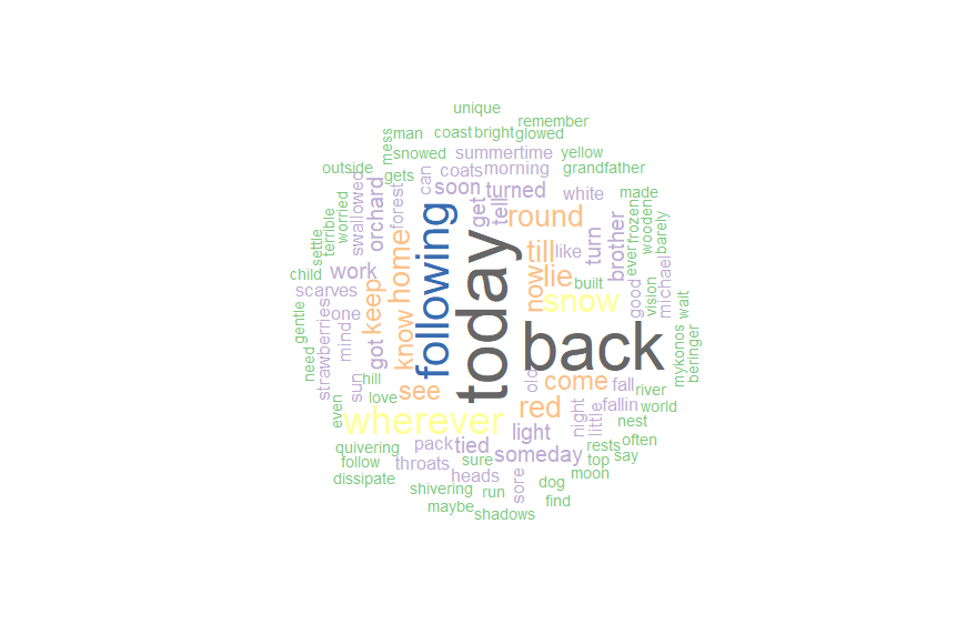
‘Today’ is the most used word by Fleet Foxes on their songs, but when we check again, Mykonos is the only song that has 18 times of word ‘today’ in it while the word ‘back’ is regularly mentioned on both hit Helplessness Blues and Ragged Wood.
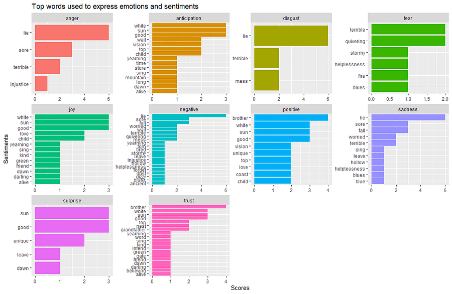
The last thing I want to do is calculate the sentiment of each songs. I’m going to use _nrc _lexicon sentiment function by Saif Mohammad and Peter Turney.
Calculate the sentiment.
song_wrd_count <- tidy_lyrics %>% count(track_title)lyric_counts <- tidy_lyrics %>%
left_join(song_wrd_count, by = "track_title") %>%
rename(total_words=n)

lyric_sentiment <- tidy_lyrics %>%
inner_join(get_sentiments("nrc"),by="word")

lyric_sentiment %>%
count(word,sentiment,sort=TRUE) %>%
group_by(sentiment)%>%top_n(n=10) %>%
ungroup() %>%
ggplot(aes(x=reorder(word,n),y=n,fill=sentiment)) +
geom_col(show.legend = FALSE) +
facet_wrap(~sentiment,scales="free") +
xlab("Sentiments") + ylab("Scores")+
ggtitle("Top words used to express emotions and sentiments") +
coord_flip()
Here’s what I got:
I also use bing lexicon sentiment function by Bing Liu and collaborators to simplify decide whether the word is positive (good) or negative (bad).
lyric_sentiment <- tidy_lyrics %>%
inner_join(get_sentiments("bing"),by="word")

lyric_sentiment %>%
count(word,sentiment,sort=TRUE) %>%
group_by(sentiment)%>%top_n(n=10) %>%
ungroup() %>%
ggplot(aes(x=reorder(word,n),y=n,fill=sentiment)) +
geom_col(show.legend = FALSE) +
facet_wrap(~sentiment,scales="free") +
xlab("Sentiments") + ylab("Scores")+
ggtitle("Positive vs Negative words") +
coord_flip()
Here’s what I got:
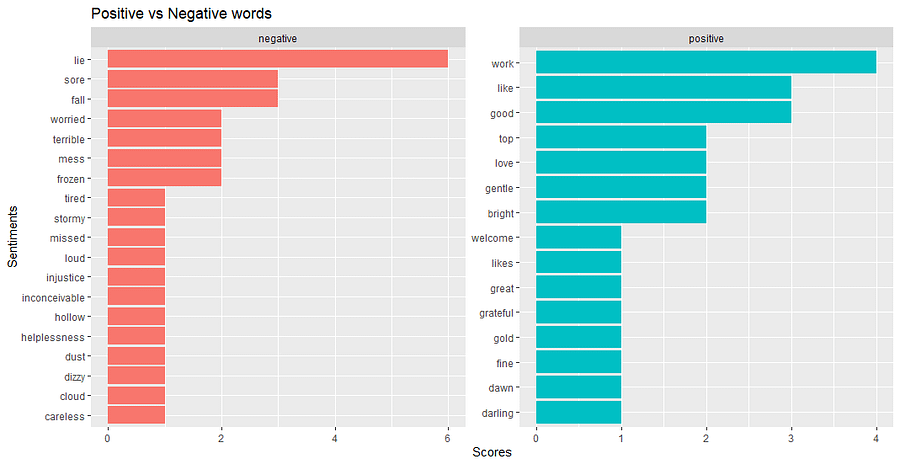
The very last thing I want to do is to make it more simple, so I make a comparison between the negative and positive words, then I visualize it on the wordcloud.
sentiment_word_bing <- tidy_lyrics  %>%
inner_join(get_sentiments("bing")) %>%
count(word, sentiment, sort = TRUE) %>%
acast(word ~ sentiment, value.var = "n", fill = 0) %>%
comparison.cloud(colors = c("#F8766D", "#00BFC4"), #c("#F8766D", "#00BFC4") max.words = 200)
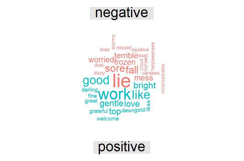
As you can see, Fleet Foxes draw the negative side of their songs using the word like lie, sore and fall. On the other side, word like work, bright and gentle makes a positive difference into their songs.
Medium: Analyzing Fleet Foxes’s Top 5 Favorite Songs Using R