Remember when we all thought 2020 would be better than 2019? It turns out that this year is much worse. From February when Covid-19 started to spread all over the world until the last couple of months, it’s been a tough year. Lot of things happen this year, the virus; people get sick and die, George Floyd, Kobe, Glenn Fredly, American Presidential Election, and much more.

We can all agree that 2020 is kind of a nightmare, but every nightmare has a break. 2020 maybe not that bad at all, especially for me and for you as fans of the Fleet Foxes. On 22 September 2020, my favorite band of all time, released their new album called Shore. Shore is the fourth album by Fleet Foxes and It is the band’s second album since regrouping in 2016 after a three-year hiatus.

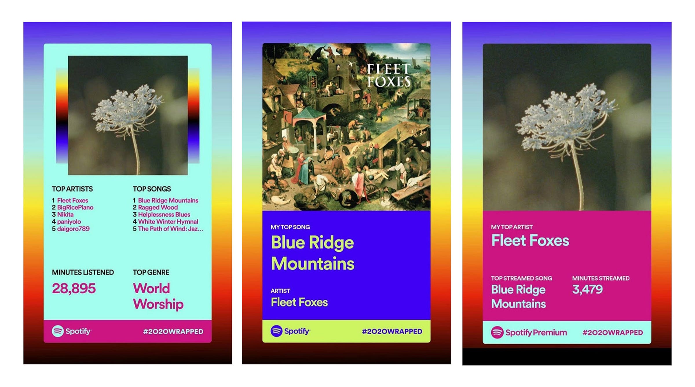
I’m a really big fan of Fleet Foxes. If you check my 2020 Spotify Wrapped, you can see the four top songs are Blue Ridge Mountains (my all time favorite), Ragged Wood, Helplessness Blues and White Winter Hymnal.

My Spotify Wrapped 2020

I’ve written an article about analyzing Fleet Foxes’s top five favorite songs before. In this article I’m going to do the same thing but I’m not going to analyze their top five favorite songs, instead I want to analyze their new album ‘Shore’.

Shore Album Tracks

I used the R programming language for the previous analysis, but for this article I will use Python. The objective of this analysis is to explore the information contained in textual documents (lyrics) within each song from the album. The album contains 15 songs, with the longest track is about 5 minutes long and the shortest track is about 2 minutes long.

Let’s jump to the code!

Still the same as the previous article, I’m using Genius library to get the data aka lyrics from Genius website database. I find that Genius also can extract not only the lyrics but also the metadata from each song or album. It’s really a useful library, but for this analysis I only need the lyrics and the title of each song.

The first thing I want to do is import all the libraries that I’ll use for the analysis.

Import the libraries

import lyricsgenius
import json
import ijson
import pandas as pd
import nltk
nltk.download('stopwords')
import re
import string
import matplotlib.pyplot as plt
%matplotlib inline
from nltk.tokenize.treebank import TreebankWordDetokenizer
from PIL import Image
from wordcloud import WordCloud
from sklearn.feature_extraction.text import CountVectorizer
from nltk.corpus import opinion_lexicon
nltk.download('opinion_lexicon')
from nltk.sentiment.vader import SentimentIntensityAnalyzer
nltk.download('vader_lexicon')

It’s pretty much a standard pack of libraries for textual documents sentiment analysis.

Generate the data

Before we can extract the data using Genius library, we need to get the token from Genius website. You can sign up and then generate your token, after that you can use your token so the API can extract the data from the Genius database.

token = "insert your token here"
genius = lyricsgenius.Genius(token)

Genius library comes with a lot of functions to extract the data. You can check all the functions on their documentation here. Since I want to get all the lyrics of each song from the album, I’ll use search_album function and then save all the extracted data into JSON format.

f = open('Lyrics_Shore.json')
data = json.load(f)g = open('Lyrics_Shore.json', 'r')
parser = ijson.parse(g)
paths = sorted(set(prefix for prefix, event, value in parser if prefix))#to check the paths
for path in paths:
    print(path)

If you print the path you’ll see that Genius not only extract the lyrics but also the metadata of the songs. In this case we have to extract the lyrics and the title from the JSON format and insert both of them into the dataframe format.

df = []
for i in data['songs']:
    df.append({'title': i["title"], 'lyrics': i["lyrics"]})shore = pd.DataFrame(df)

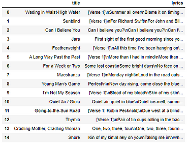
Once it’s done, you’ll get a dataframe with two columns. One is the title of each song and the other is the lyrics of each song.

Dataframe contains Title and Lyrics

Since the lyrics are still in a dirty format then our next step is doing the cleansing to remove unnecessary string from the lyric.

Cleansing

I’m going to remove the punctuation, remove unnecessary text like Verse, Chorus, Outro, convert the text to lowercase, split the words, and then remove the stopwords.

stopword = nltk.corpus.stopwords.words('english')
def remove_stopwords(text):
    text=[word for word in text if word not in stopword]
    return textdef remove_punctuation(text):
    no_punct=[words for words in text if words not in string.punctuation]
    words_wo_punct=''.join(no_punct)
    return words_wo_punctdef detokenize(text):
    de = TreebankWordDetokenizer().detokenize(text)
    return deshore['lyrics']=shore['lyrics'].apply(lambda x: remove_punctuation(x))
shore['lyrics'] = shore['lyrics'].str.replace(r'Verse', '')
shore['lyrics'] = shore['lyrics'].str.replace(r'Chorus', ' ')
shore['lyrics'] = shore['lyrics'].str.replace(r'Outro', ' ')
shore['lyrics'] = shore['lyrics'].str.replace(r'\n', ' ')
shore['lyrics'] = shore['lyrics'].str.replace(r'\u2005', ' ')
shore['lyrics'] = shore['lyrics'].str.replace('\d+', '')
shore['lyrics'] = shore['lyrics'].str.lower()
shore['lyrics'] = shore['lyrics'].str.split()
shore['filtered_words'] = shore['lyrics'].apply(lambda x: remove_stopwords(x))
shore['clean_lyrics'] = shore['filtered_words'].apply(lambda x: detokenize(x))

After all done, now you can use the data to the analysis because now the lyrics are clean and ready to use. The first thing I want to do is count the words from each song.

Count of words

shore['words_count'] = shore['lyrics'].str.len()
shore = shore.sort_values('words_count')

After that, I visualize it using Matplotlib.

shore.plot.barh(x='title', y='words_count', figsize=(9,6), colormap='summer', title='Number of Words for each Title');

Number of Words for each Title

As you can see, Sunblind has the most words compared to other songs in the album, while Thymia has the least words. The next thing I want to do is using vocabulary to find the number of unique words used by each song (lexical richness).

Lexical richness

Dividing the number of words used with the vocabulary gives us a measure of the lexical richness of each artist (i.e., what proportion of the words used in the songs are distinct).

shore['filtered_words_count'] = shore['filtered_words'].str.len()
shore['lexical_richness'] = shore['filtered_words_count']/shore['words_count']*100
shore = shore.sort_values('lexical_richness')
shore.plot.barh(x='title', y='lexical_richness', figsize=(9,6), colormap='Wistia', title='Lexical Richness for each Title')

Lexical Richness for each Title

The result after dividing the number of words used with the vocabulary, as you see, Quiet Air/Gioia has the most lexical richness while Sunblind dropped to the fourth rank even though it has the most words. On the other hand, even though Thymia has the least words, it actually has more lexical richness compared to other songs in the album.

Wordcloud

Once we know the number of words and lexical richness within each song, now I want to visualize all the most used words from the album (all songs). I’ll use wordcloud to visualize all the words, but before I do that, I have to count all the words from each song and convert it to a vector.

I’m using sci-kit learn countvectorizer to count the frequency of each word.

X = shore['clean_lyrics']\
vectorizer = CountVectorizer()\
text_vec = vectorizer.fit_transform(X.values.astype('U'))\
word_count = pd.DataFrame(text_vec.toarray(), columns=vectorizer.get_feature_names())word_list = vectorizer.get_feature_names()\
count_list = text_vec.toarray().sum(axis=0)\
word_freq = dict(zip(word_list,count_list))

And then, I visualize it using wordcloud.

wcp = WordCloud(background_color="white",width=1000,height=1000, max_words=100,relative_scaling=0.5,normalize_plurals=False).generate_from_frequencies(word_freq)
plt.figure(figsize=(9,6))
plt.imshow(wcp)
plt.axis('off')
plt.show()

Wordcloud for most used words from the album

“one” and “want” are the most used words, followed by “water”, “walk”, and “never”. It’s obvious since the word “water” is regularly mentioned on the first two track, Wading In Waist-High Water and Sunblind.

Sentiment Analysis

I’ll use two sentiment analysis techniques. First, I’ll use Vader Sentiment Analysis to calculate polarity scores which will return four scores: positive, neutral, negative, and compound. For this analysis, I’ll ignore the compound score and will focus more on positive, neutral, and negative scores.

For the second analysis, I’ll use NRC Opinion Lexicon to calculate the lyrics based on the weight or category of each word. Similarly to Naive Bayes, this sentiment analysis will calculate each word as an independent feature and ignore the whole context of the words.

Vader Sentiment Analysis

analyzer = SentimentIntensityAnalyzer()
shore['compound'] = [analyzer.polarity_scores(x)['compound'] for x in shore['clean_lyrics']]
shore['neg'] = [analyzer.polarity_scores(x)['neg'] for x in shore['clean_lyrics']]
shore['neu'] = [analyzer.polarity_scores(x)['neu'] for x in shore['clean_lyrics']]
shore['pos'] = [analyzer.polarity_scores(x)['pos'] for x in shore['clean_lyrics']]sentiment = pd.DataFrame()
sentiment = shore[['title', 'neg', 'neu', 'pos']]
sentiment.plot.bar(x='title', stacked=True, figsize=(9,6), color={'pos': 'green', 'neg': 'red', 'neu': 'blue'})
plt.show()

Vader Sentiment Analysis

I use three scores from the analyzer. As you can see on the stacked bar above, the red bar represents the score of negative sentiment, the blue bar represents the score of neutral sentiment, and the green bar represents the score of positive sentiment.

Sunblind has the most positive sentiment score, while Going-to-the-sun Road has the lowest score. On the contrary, Quiet Air/Gioia has the most negative sentiment score, while Sunblind, I’m Not My Season, and Can I Believe You share the same low negative sentiment score.

NRC Opinion Lexicon

pos_list=set(opinion_lexicon.positive())
neg_list=set(opinion_lexicon.negative())def sentiment(sentence):
  senti=0
  words = [word for word in sentence]
  for word in words:
    if word in pos_list:
      senti += 1
    elif word in neg_list:
      senti -= 1
  return sentishore['sentiment']=shore['filtered_words'].apply(sentiment)
shore['is_positive'] = shore['sentiment'] > -0
shore[['title', 'sentiment']].plot(x='title', kind='bar',  title='Sentiment for each Title using NRC', figsize=(9,6), legend= False, color=[shore.is_positive.map({True: 'yellow', False: 'red'})])

NRC Opinion Lexicon

As you can see on the barplot above, since NRC calculates each word as an independent feature so it doesn’t really care about the context of the words or lyrics itself. The more negative classified words appear in a sentence then NRC will assume that the whole sentence is actually negative even though is not actually negative, in the perspective of human linguistics.

The results of the NRC Opinion Lexicon revealed that there are ten songs from the album classified as songs with higher negative sentiment, while the rest have more positive sentiment. The negative sentiment songs include Quiet Air/Gioia, Jara, Maestranza, Can I Believe You, Wading in Waist-High Water, and several others.

Positive and Negative Words

The very last thing I want to do is to make a comparison between positive and negative words that appear in every song on the album. The comparison is actually built by classifying positive and negative words and then visualizing both of the classifications with wordcloud.

#pos neg words classified
pos_dic = list(pos_list)
neg_dic = list(neg_list)a = shore['filtered_words']
pos_word = []
neg_word = []
all_words = []
for sublist in a:
    for item in sublist:
        all_words.append(item)for word in all_words:\
    if word in pos_dic:
        pos_word.append(word)
    elif word in neg_dic:
        neg_word.append(word)

Wordcloud for the positive words:

# wordcloud for positive words
unique_string=(" ").join(pos_word)
wcp = WordCloud(background_color="white",width=2000,height=1000, max_words=1000,relative_scaling=0.5,normalize_plurals=False, colormap="summer").generate(unique_string)
plt.figure(figsize=(10,8))
plt.imshow(wcp)
plt.axis('off')
plt.show()

Wordcloud for Positive Words

Wordcloud for the negative words:

# wordcloud for negative words
unique_string=(" ").join(neg_word)
wcp = WordCloud(background_color="white",width=2000,height=1000, max_words=1000,relative_scaling=0.5,normalize_plurals=False, colormap="RdGy").generate(unique_string)
plt.figure(figsize=(10,8))
plt.imshow(wcp)
plt.axis('off')
plt.show()

Wordcloud for Negative Words

As you can see, Fleet Foxes draw the negative side of their new album using the words like “wrong”, “devil”, “weak”, and “heartless”. On the other hand, words like “warm”, “well”, “quiet”, and “love” make a positive difference in their new album.

Medium: Analyzing Fleet Foxes New Album ‘Shore’ Using Python